Chapter 13: Designing a Search Autocomplete System

note

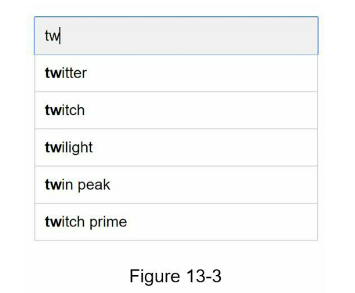
Autocomplete (also called typeahead or search-as-you-type) shows suggested queries while users type. It is widely used in systems like Google Search or Amazon. The interview question is: design a system that returns the top-k most popular search queries given a prefix.

---

Step 1 - Understand the problem and establish design scope

Candidate: Is the matching only supported at the beginning of a search query or in the middle as well?
Interviewer: Only at the beginning of a search query.
Candidate: How many autocomplete suggestions should the system return?
Interviewer: 5
Candidate: How does the system know which 5 suggestions to return?
Interviewer: This is determined by popularity, decided by the historical query frequency.
Candidate: Does the system support spell check?
Interviewer: No, spell check or autocorrect is not supported.
Candidate: Are search queries in English?
Interviewer: Yes. If time allows at the end, we can discuss multi-language support.
Candidate: Do we allow capitalization and special characters?
Interviewer: No, we assume all search queries have lowercase alphabetic characters.
Candidate: How many users use the product?
Interviewer: 10 million DAU.

Requirement

1. Speed: Results must appear within ~100 ms.
2. Relevance: Suggestions must match the prefix.
3. Ranking: Sorted by popularity (query frequency).
4. Scalability: Handle millions of users and high query per second (QPS).
5. Availability: Must stay online despite failures.

Estimation:

• Assume 10 million daily active users (DAU).
• An average person performs 10 searches per day.
• 20 bytes of data per query string:
  • Assume we use ASCII character encoding. 1 character = 1 byte
  • Assume a query contains 4 words, and each word contains 5 characters on average.
  • That is 4 x 5 = 20 bytes per query.
• On average, 20 requests are sent for each search query. For example, the following 6 requests are sent to the backend by the time you finish typing “dinner”.
  • search?q=d
  • search?q=di
  • search?q=din
  • search?q=dinn
  • search?q=dinne
  • search?q=dinner
• ~24,000 query per second (QPS) = 10,000,000 users * 10 queries / day * 20 characters / 24 hours / 3600 seconds.
• Peak QPS = QPS * 2 = ~48,000
• Assume 20% of the daily queries are new. 10 million * 10 queries / day * 20 byte per query * 20% = 0.4 GB.
• => This means 0.4GB of new data is added to storage daily.

---

Step 2 – High-Level Design

Two main services:

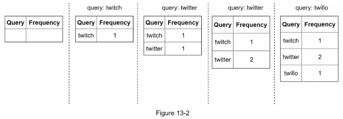
1. Data Gathering Service – collects queries, aggregates them, and stores frequency data.

2. Query Service – given a prefix, returns the top-5 most searched queries.

---

Step 3 – Deep Dive Design

Core Data Structure: Trie

• Trie (pronounced “try”) is a tree-like data structure that can compactly store strings.

• The main idea of trie consists of the following:

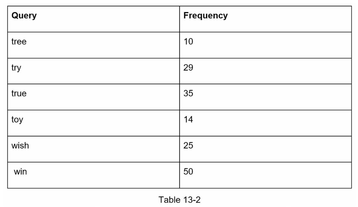
  • A trie is a tree-like data structure.
  • The root represents an empty string.
  • Each node stores a character and has 26 children, one for each possible character. To save space, we do not draw empty links.
  • Each tree node represents a single word or a prefix string.

• How does autocomplete work with trie? Before diving into the algorithm, let us define some terms.

  • p: length of a prefix
  • n: total number of nodes in a trie
  • c: number of children of a given node

• Steps to get top k most searched queries are listed below:

  1. Find the prefix. Time complexity: O(p).
  2. Traverse the subtree from the prefix node to get all valid children. A child is valid if it can form a valid query string. Time complexity: O(c)
  3. Sort the children and get top k. Time complexity: O(clogc)

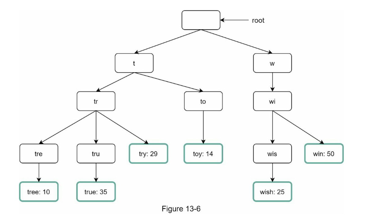
• Example in Figure 13-7: a user types “tr” in the search box. The algorithm works as follows:

  • Step 1: Find the prefix node “tr”.
  • Step 2: Traverse the subtree to get all valid children. In this case, nodes [tree: 10], [true: 35], [try: 29] are valid.
  • Step 3: Sort the children and get top 2. [true: 35] and [try: 29] are the top 2 queries with prefix “tr”.
  • The time complexity of this algorithm is the sum of time spent on each step mentioned above: O(p) + O(c) + O(clogc)

• Optimizations:

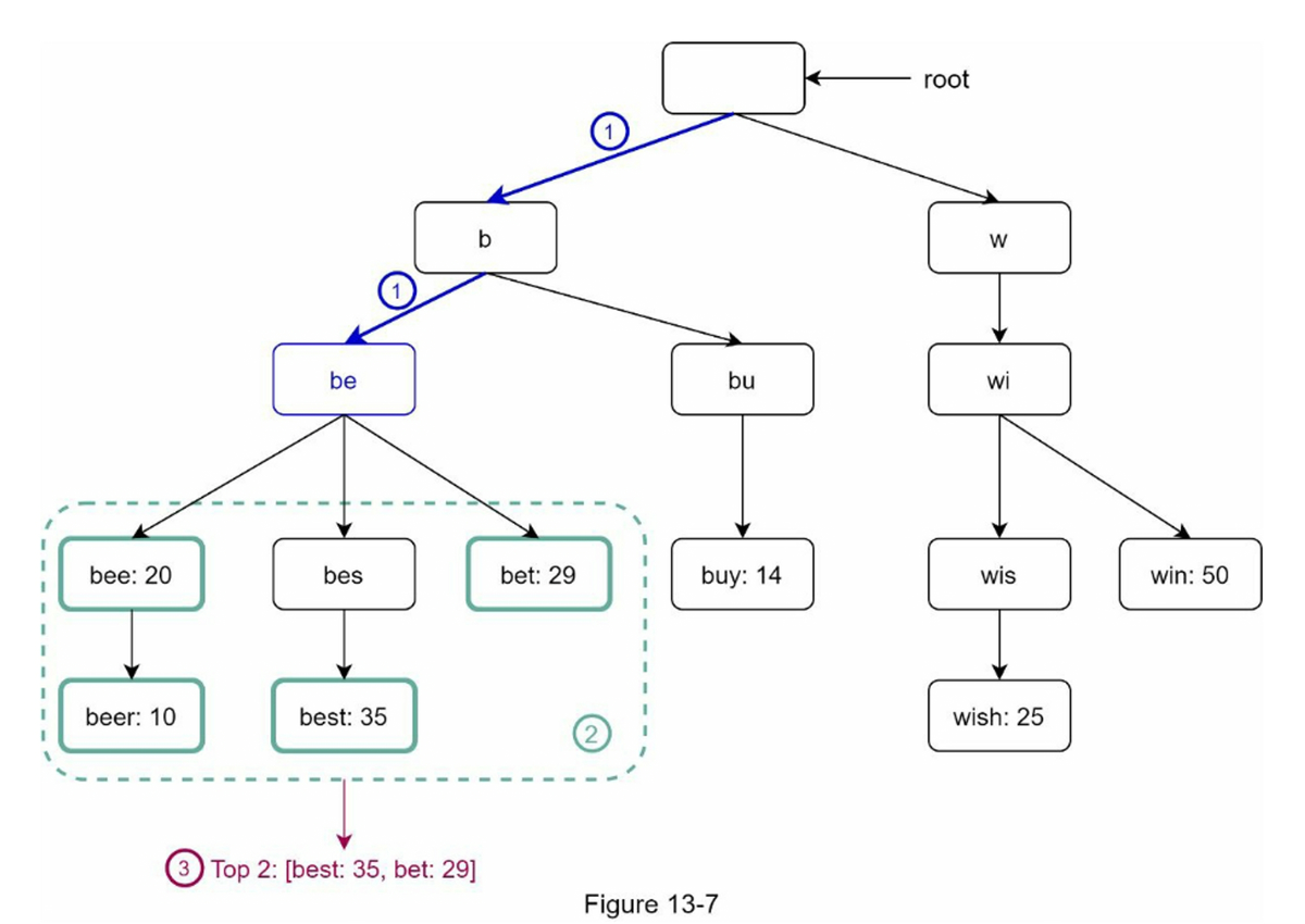
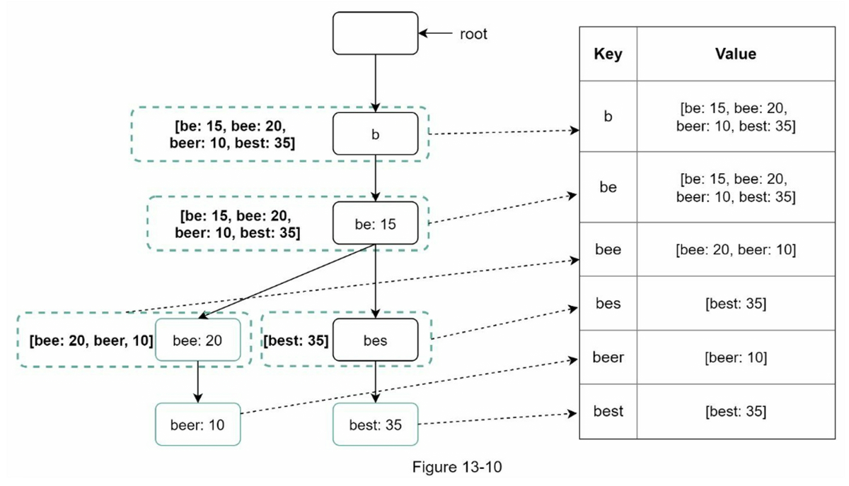
  • Limit prefix length (constant-time lookup): Users rarely type a long search query into the search box. Thus, it is safe to say p is a small integer number, say 50. If we limit the length of a prefix, the time complexity for “Find the prefix” can be reduced from O(p) to O(small constant), aka O(1).
  • Cache top queries at each node (trade space for time).
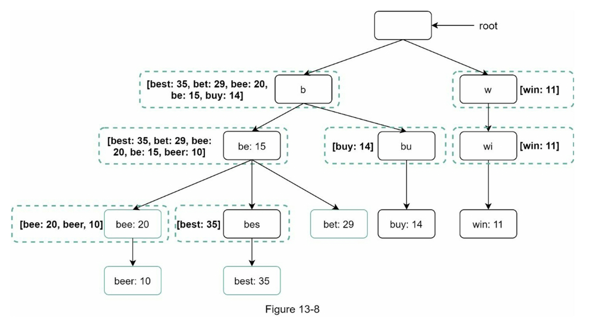
  • After applying those two optimizations:
    1. Find the prefix node. Time complexity: O(1)
    2. Return top k. Since top k queries are cached, the time complexity for this step is O(1)
  • As the time complexity for each of the steps is reduced to O(1), our algorithm takes only O(1) to fetch top k queries.

Data Gathering Service

• Before, data is updated in real-time. This approach is not practical for the following two reasons:
  1. Users may enter billions of queries per day. Updating the trie on every query significantly slows down the query service.
  2. Top suggestions may not change much once the trie is built. Thus, it is unnecessary to update the trie frequently.
• Redesigned data gathering service:
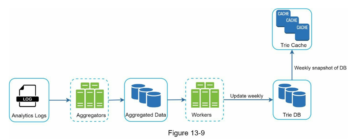
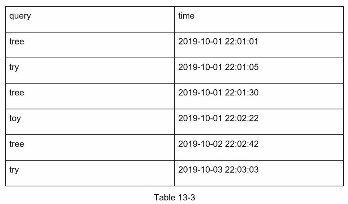
  • Analytics Logs: Store raw data of search queries. Logs are append-only and not indexed.
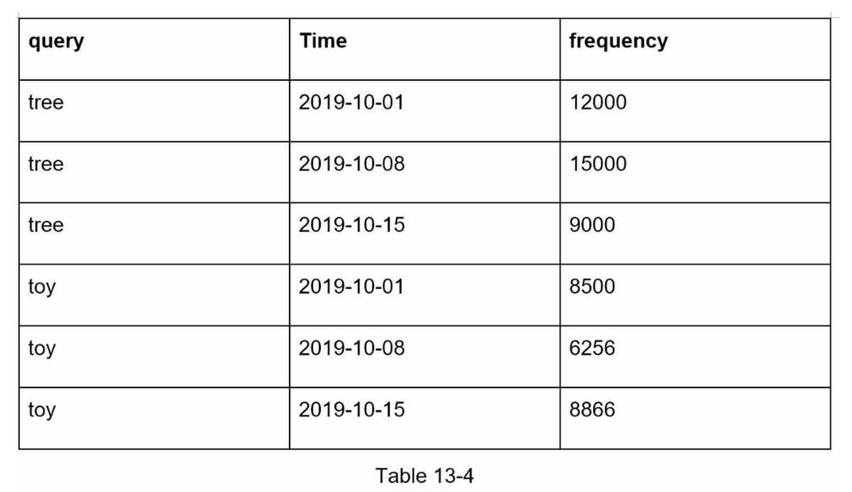
  • Aggregators: Logs are very large and not in the right format, so we aggregate them.
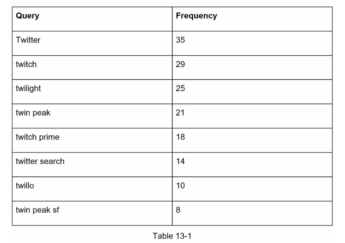
  • Aggregated Data:
  • Workers: Workers are a set of servers that perform asynchronous jobs at regular intervals. They build the trie data structure and store it in Trie DB.
  • Trie Cache: Trie Cache is a distributed cache system that keeps trie in memory for fast read. It takes a weekly snapshot of the DB.
  • Trie DB: Trie DB is the persistent storage. Two options are available to store the data:
    1. Document store: Like MongoDB
    2. Key-value store: A trie can be represented in a hash table form by applying the following logic:
    • Every prefix in the trie is mapped to a key in a hash table.
    • Data on each trie node is mapped to a value in a hash table.
    • PS. If you are unclear how key-value stores work, refer to Chapter 6: Design a key-value store.

Query Service

• Query Service Design:
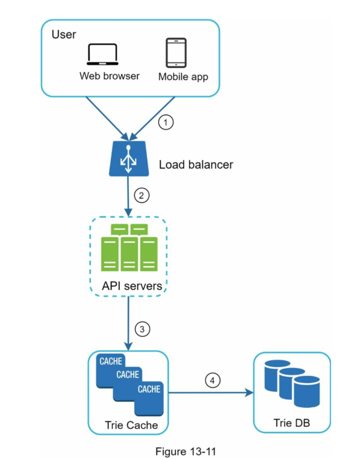
  1. A search query is sent to the load balancer.
  2. The load balancer routes the request to API servers.
  3. API servers get trie data from Trie Cache and construct autocomplete suggestions for the client.
  4. In case the data is not in Trie Cache, we replenish data back to the cache. This way, all subsequent requests for the same prefix are returned from the cache. A cache miss can happen when a cache server is out of memory or offline.
• lightning-fast speed optimizations:
  1. AJAX request: Sending/receiving a request/response does not refresh the whole web page.
  2. Browser caching
  3. Data sampling: For instance, only 1 out of every N requests is logged by the system.

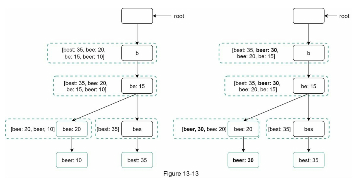
Trie Operations

• Create: workers build trie from aggregated logs.
• Update: replace weekly, or update nodes (slower).
  • Option 1: Update the trie weekly. Once a new trie is created, the new trie replaces the old one.
  • Option 2: Update individual trie node directly.
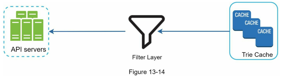
• Delete: use filter layer to remove offensive/unsafe suggestions.

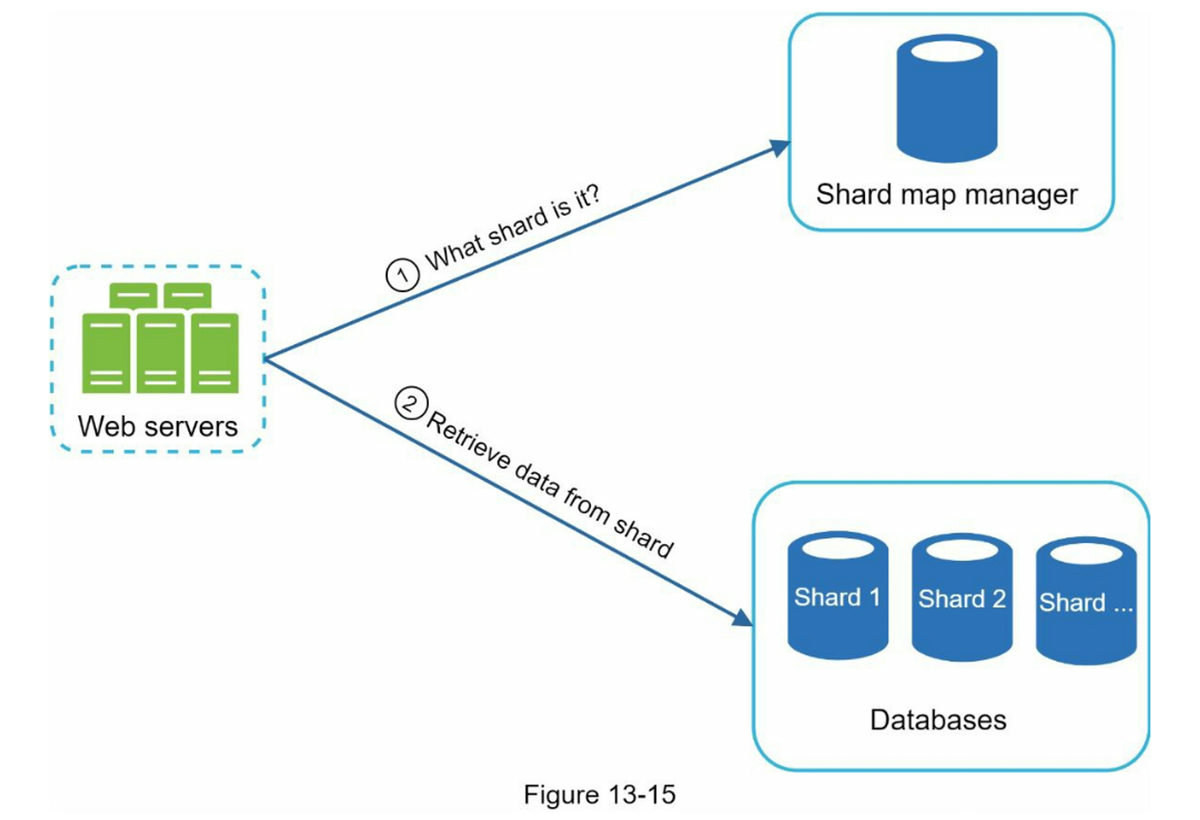
Scaling

• Shard data across servers (e.g., by first character).
• Adjust shard ranges dynamically to avoid uneven distribution. For example, if there are a similar number of historical queries for ‘s’ and for ‘u’, ‘v’, ‘w’, ‘x’, ‘y’ and ‘z’ combined, we can maintain two shards: one for ‘s’ and one for ‘u’ to ‘z’.

---

Step 4 – Extensions

• Multi-language support: use Unicode in trie.
• Country-specific trends: build separate tries per region; distribute with CDNs.
• Real-time trending queries...some tips:
  • Autocomplete requires fast response and efficient data structures.
  • Trie + caching makes O(1) query response possible.
  • Batch aggregation balances performance and freshness.
  • Scalability and filtering are critical for production readiness.